Formally deriving programs from specifications using Lean 4 in the Bird-Meertens style
This page describes the systematic derivation of an efficient algorithm from an obviously correct but inefficient specification using formally verified transformations, as illustrated in the code below (from Kadane.lean). With the recent advances in AI coding agents and the automation of proofs using AI theorem provers, this inspiring idea from the 1980s deserves another look.
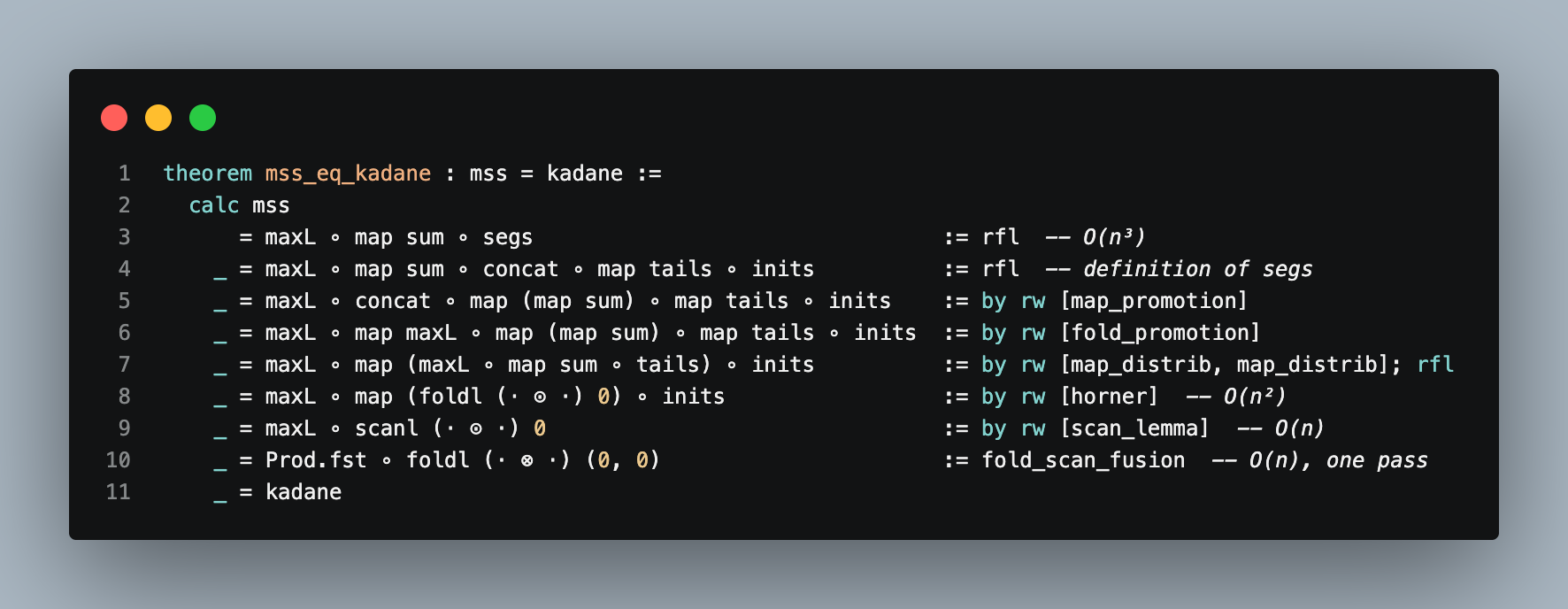
Tap or click the image to open it at full resolution.
The problem: give me a list of integers and ask for the contiguous segment with the largest
sum, and the obvious thing to do is to try every segment, add each one up, and
keep the biggest. For [-2, 1, -3, 4, -1, 2, 1, -5, 4] the winner is
[4, -1, 2, 1], which sums to 6. This brute force approach is easy to believe
but it costs O(n³). Kadane’s algorithm gets the same answer in a single O(n)
pass over the list, but it is not at all obvious why it works. Richard Bird
showed how to calculate Kadane’s algorithm from the obvious specification,
one algebraic law at a time, in Algebraic Identities for Program Calculation
(The Computer Journal, 1989, §8). It is the poster child of the Bird–Meertens
formalism (affectionately known as Squiggol), and Wikipedia shows the same
derivation in its
Bird–Meertens formalism
article.
Here I replay Bird’s derivation in Lean 4. The specification is at the top, Kadane’s algorithm is at the bottom, and every step in between is a law that Lean has checked (no hand waving, no “it is easy to see that”). The bit I like best is that every line of the derivation is itself a runnable program, so we can time each one and watch the complexity drop as the laws are applied. Everything uses plain core Lean with no Mathlib.
The Derivation
The whole derivation is one calc block, mss_eq_kadane in
Kadane.lean. Each line is a program and each
step cites exactly one law, just like Bird’s figure.
  maxL ∘ map sum ∘ segs                                 O(n³)
= maxL ∘ map sum ∘ concat ∘ map tails ∘ inits           definition of segs
= maxL ∘ concat ∘ map (map sum) ∘ map tails ∘ inits     map promotion
= maxL ∘ map maxL ∘ map (map sum) ∘ map tails ∘ inits   fold promotion
= maxL ∘ map (maxL ∘ map sum ∘ tails) ∘ inits           map distributivity
= maxL ∘ map (foldl (⊙) 0) ∘ inits                      Horner's rule     O(n²)
= maxL ∘ scanl (⊙) 0                                    scan lemma        O(n)
= fst ∘ foldl (⊗) (0, 0)                                fold–scan fusion  O(n)
The first line is the specification: take all the segments (every tail of
every prefix), sum each one, and take the maximum. The next four steps just
shuffle the plumbing around without changing the cost. Horner’s rule is where
the magic happens: the best sum of a segment ending at some point can be
computed with a left fold of a ⊙ b = max (a + b) 0, which saves a factor of
n. The scan lemma notices that folding over every prefix is just a scanl,
which saves another factor of n. Finally, fold–scan fusion carries the
running maximum along with the fold, so we never build the intermediate list
at all. The pair operator is (u, v) ⊗ x = (max u w, w) where w = v ⊙ x,
and that last line is Kadane’s algorithm.
A few details that matter in the Lean version:
- The lists hold
Intvalues. The empty segment counts as a segment, so the answer is never negative (for[-3, -1, -2]the answer is 0). maxLfoldsmaxstarting from0, which makes0its unit. This is what lets the empty segment and the laws play nicely together.- The laws used in the middle of the pipeline carry a trailing
∘ gso thatrwcan find them inside a longer composition.
Running Times
The benchmark in bench/KadaneBench.lean runs every
line of the calc block on random lists of growing length and times each one.
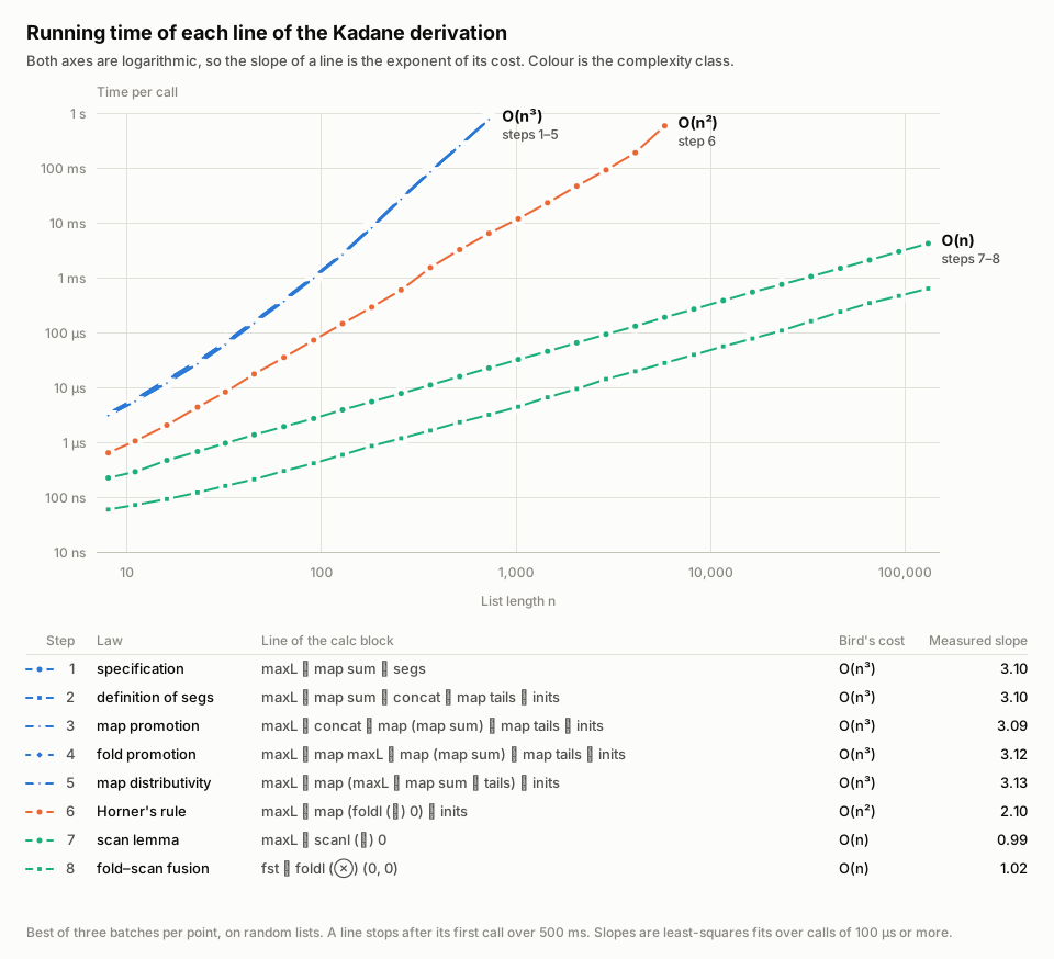
Both axes are logarithmic, so a program that costs c·nᵏ shows up as a
straight line with slope k. The three complexity classes in Bird’s
derivation turn up as three slopes, which I find very satisfying to see.
- Steps 1 to 5 sit right on top of each other. Their four laws move things around but leave the cost unchanged.
- Horner’s rule knocks off a factor of
n, and the scan lemma knocks off another. - Fold–scan fusion is still O(n) but it runs about 7 times faster than the scan, because it never builds the intermediate list.
- At n = 512 the specification takes 271 ms, while the last line takes 2.4 µs. That is about 110,000 times faster for the same answer.
| Step | Law | Bird’s cost | Measured slope | n = 512 | Largest n | Time there |
|---|---|---|---|---|---|---|
| 1 | specification | O(n³) | 3.10 | 271 ms | 724 | 807 ms |
| 2 | definition of segs | O(n³) | 3.10 | 270 ms | 724 | 807 ms |
| 3 | map promotion | O(n³) | 3.09 | 268 ms | 724 | 803 ms |
| 4 | fold promotion | O(n³) | 3.12 | 266 ms | 724 | 799 ms |
| 5 | map distributivity | O(n³) | 3.13 | 265 ms | 724 | 796 ms |
| 6 | Horner’s rule | O(n²) | 2.10 | 3.39 ms | 5,793 | 611 ms |
| 7 | scan lemma | O(n) | 0.99 | 16.5 µs | 131,072 | 4.39 ms |
| 8 | fold–scan fusion | O(n) | 1.02 | 2.42 µs | 131,072 | 661 µs |
The slopes of the first six lines come out a little above 3 and 2. My guess
is that inits keeps all n²/2 prefix cells alive, so the memory traffic
grows a bit faster than the operation count.
You might worry that the benchmark is timing a slightly mistyped copy of a
line rather than the real thing. It is not: lines_eq_mss proves that every
timed program equals mss, and its proof replays the same laws. Each run also
checks that all eight lines agree on every input, just to be sure.
Each point is the fastest of three batches, where a batch repeats the call
until it lasts at least 20 ms. A line is dropped after its first call that
takes over 500 ms (which is why the cubic lines give up early). A slope is a
least-squares fit of log t against log n, using only calls of 100 µs or
more.
These numbers come from a single run on a 2.60 GHz Intel Xeon (a GCP VM) with Lean 4.28.0. Your absolute times will be different on another machine, but the slopes should hardly change. To run it yourself, from the root of the repository:
lake exe kadane_bench        # takes about 40 seconds
lake exe kadane_bench 50     # stop each line at 50 ms instead of 500 ms
This writes every measurement to
bench/kadane_timings.csv and redraws both SVG
plots (a light one and a dark one, picked to match your GitHub theme).
AI Coding and AI Proofs
This approach of deriving programs from specifications was a great idea from the 1980s which was perhaps ahead of its time but I think has now found relevance in the age of AI coding. Specifically, AI coding agents and AI theorem provers can now work to synthesize and optimize code from specifications or draft implementations into efficient and correct by construction code (the guarantee comes from the checked proofs, not from the agent).
Previously the level of skill required and the laborious details needed to perform the proofs for practical programs made this approach difficult to apply. Now AI coding and automatic AI theorem proving advances mean we should look again at this approach for synthesizing code in a manner that still retains some form of comprehension for humans, given by the stepwise refinement steps which act as a kind of explanation of how code has been transformed and synthesized.
Finding out more and some other related work
The GitHub repo Algebra of Programming in Agda: Dependent Types for Relational Program Derivation contains an Agda implementation of a library inspired by the Algebra of Programming as described in a book by Richard Bird and Oege de Moor (Oege is now famous for GitHub Copilot and XBOW).
Jeremy Gibbons has written an article about The School of Squiggol: A History of the Bird−Meertens Formalism.
Building
The toolchain is pinned in lean-toolchain (Lean
v4.34.1) and nothing outside core Lean is needed. Run these from the root of
the repository.
lake build                   # checks the derivation
lake exe kadane_bench        # the timings and plots
You can find all the code used for this article at https://github.com/satnam6502/bird-meertens.